Description
University of Essex, 2018-19
Dissertation submitted in partial fulfilment of the requirements for the award of MSc in Business Analytics
Abstract
Big data analytics (BDA) is no longer a competitive advantage, but a compulsory ability to endure in an ecosystem increasingly attentive to customer behaviour. In this context, few industries offer such an abundance of raw customer data as e-commerce, where is possible to explore why users make many decisions and judgments. One of most commonly used feature in e-commerce is the online customer review rating (OCR), a form of electronic word of mouth (eWOM) that can reduce the unfamiliarity risk in purchase decision, and also seen as an essential index of overall customer satisfaction. Although the idea of OCRs as a sales driver being well researched, little is discussed about the factors coming from the side of the seller that drive the OCRs themselves. This research, as an alternative, uses OCR as the predicted variable, testing if the different ways the product and order were placed may impact on final consumer satisfaction (measured by the OCR). To investigate this relationship, the research conducts an Exploratory Data Analysis (EDA) of order attributes (such as delivery time, description length and price) contained in a data set of 100,000 transactions made through a Brazilian marketplace called Olist. Next, the research uses the attributes to predict the OCR through Linear and Ordinal Logistic regressions, as well as through Random Forest regression and classification models. The Random Forest classifier, in particular, produces a very reliable prediction, with an accuracy of 1.00 for OCRs rated as 1, 4 and 5, and an accuracy of 0.99 for OCRs rated as 2 and 3. The attribute weights and correlations are somewhat validated, and the outcomes may contribute to future work of scholars and entrepreneurs in the field of consumer behaviour, product management, and data analysis.
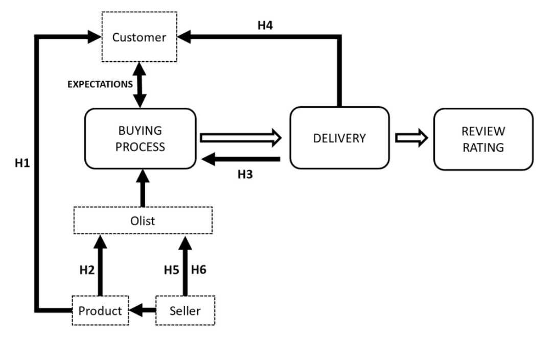
The research tries to understand if the product category or the order organisation and execution might have an influence on customer satisfaction by creating some expectations, that will be fulfilled or not. Being a very general investigation, it is further subdivided into six hypotheses to facilitate the experiment according to the different attributes collected — from how the product is displayed up to when it is delivered. Then, a model is developed for predicting which score (OCR) the consumer would give according to the information from these attributes. Therefore, the research question is:
“Does particular product characteristics and order structures impact on the final customer satisfaction (measured by the OCR)?”
Research hypotheses:
- H1: Product categories have biases towards the online customer review rating (OCR)
- H2: An increase in the product price negatively impacts the online customer review rating (OCR)
- H3: An increase in the delivery price negatively impacts the online customer review rating (OCR)
- H4: An increase in the delivery time negatively impacts the online customer review rating (OCR)
- H5: An increase in the description size positively impacts the online customer review rating (OCR)
- H6: An increase in the number of photos positively impacts the online customer review rating (OCR)

Data Cleaning and Preprocessing
The data set information was collected from about 100,000 orders made through a Brazilian marketplace called Olist from 2016 to 2018. Olist, besides having its own e-commerce, registers its sellers in a system that connects to other large e-commerce in Brazil, such as Amazon, Carrefour and Mercado Livre (Olist Serviços Digitais Ltda, 2016-2018). It is a public data set, provided by Olist itself through an Attribution-NonCommercial-ShareAlike 4.0 International (CC BY-NC-SA 4.0) license of use, and available at the online data scientists community Kaggle, owned by Google LLC. At the time of this dissertation, the database is in its Version 7, and it was last updated on November 29, 2018.
All features’ One-Sample T-test had p-value > 0.05, and therefore, we accept the null hypothesis that the sample mean is not significantly different from the population mean. It should be noted here that it was challenging to find a normal distribution within most features, including those extracted for this study.
Several highly significant Tests of Normality (both Kolmogorov-Smirnov and Shapiro-Wilk) were performed, with Q-Q chart points tending to pull away from the line that provides the expected normal distribution, indicating that the features are not normally distributed.
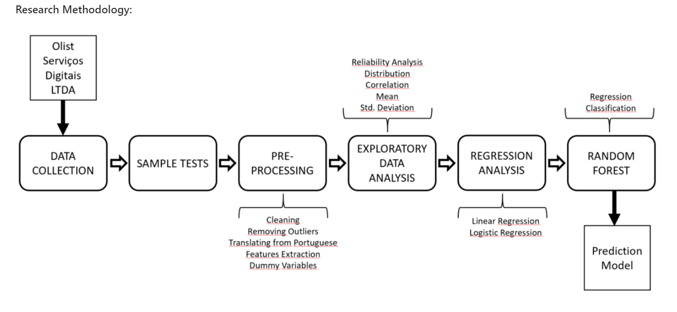
The first step was to merge the original data set with a parallel set called product_category_name_english, and then replace the information from the original category feature, to translate product categories into English. Being a Brazilian company, the original data was in Portuguese.
There are, in fact, some outliers in all features. This was detected through visual analysis by boxplots and through the Z-score function, for better describing the relationship of the data with its Mean and Standard Deviation. Data points with Z-score values greater than the threshold value of 3 and lesser than -3 have been adequately eliminated, resulting in an updated data set of 89,134 orders. Both the developed Regression Analysis and Random Forest were tested with data sets with and without outliers, and in both, the performance was increased in the data set without outliers.
Exploratory Data Analysis
Through the process of data analysis, data is collected and analysed to answer questions, test hypotheses, or disprove theories (Judd & McClelland, 1989).
Two Reliability Analysis for detecting multi-correlating features were performed for the extraction of a Cronbach’s α (alpha), which helps to measure internal consistency and uni-dimensionality (Tavakol & Dennick, 2011). The first included the variables prod_value, delivery_value and total_value, and the second included delivery_est_time, delivery_act_time, and delivery_precision. The goal was to understand if a dimension reduction through Factor Analysis would be useful to extract some set of hidden variables explaining their relationship. The first test group resulted in a Cronbach value greater than 0.7, meaning the variables have a high correlation.
A Factor Analysis was performed and extracted two components, which one of them with an eigenvalue explaining 75% of the relationship (basically representing prod_value and total_value). The high correlation, although ignored at the moment, showed that one of these variables should be excluded from the Regression Analysis ahead. The second test group resulted in a Cronbach value of less than 0.7, which is treated as a low correlation between variables (Tavakol & Dennick, 2011).
The purpose of the research’s exploratory data analysis (EDA) is not to understand the entire data set, but only the feature’s correlations with the dependent variable online customer rating (OCR). Scatterplot, boxplot, value distributions by Review Score’s means and analysis of variance (ANOVA) were used for this purpose through Python groupby and describe functions, IBM SPSS statistical software, and Tableau for data visualisation.
As for the relationship between reviews and delivery time, it is possible to see much more clearly that both the current average delivery time (represented by the variable delivery_act_time) and the average delivery precision (delivery_precision) influence the score attributed by the consumer, as explained by the higher coefficient of correlation calculated before. Estimated time is not represented here because it has a lower correlation, possibly meaning that the time expected to be delivered doesn’t impact much at the time of purchase, only after it, while waiting for the real delivery. It is clear, indeed, that low review scores concentrate more late orders than the high scores.
The mean average of the delivery actual time assigned to 1-star orders is 16.63 days, and as it decreases, it moves to a higher OCR, reaching 10.69 days in 5 stars. The minimum and maximum days also change, reaching 0.53 day in 5-stars reviews and 1.07 days in 1-star reviews. The relationship of the OCR with delivery precision is reversed, where the mean average of a product being delivered in advance is 12.77 days in 5-stars reviews and 7.55 days 1-star reviews. However, in all ratings there are delays, reaching the maximum of 18.92 days late in 5-stars reviews and 19.07 in 1-star review.
Models
To verify the correlation between attributes and OCRs, this study performs predictions that linearly depends on the explanatory data we have, by means of a Linear Regression Analysis (Glasserman, 2011) and by extracting the ratio of variance explained by the regression model, known as the coefficient of determination, or R-squared (Rao, 1973).
Later on, the research explains the possible correlations through a regression method specifically used for arbitrary scaled (a.k.a. ordinal) dependent variables, such as the research’s OCR. Known as Ordinal Logistic Regression, this type of regression can also be considered a classification method (Winship & Mare, 1984).
Next, to validate whether the relationship explained by the earlier regression analyses would work with new information, this research attempts to perform some predictions. It develops a supervised learning classification model using the known observations contained in a separate training set to predict the rating class of given data points. Random Forest (a particular method of ensemble learning) is chosen because it performs very well compared to the other classifiers, is robust against over-fitting and very user-friendly, being widely used both for regression and classification problems from this type of independently-constructed tabular data set (Hastie et al., 2009; Breiman, 2001; Elite Data Science, 2019; Ho, 1995; Thanh Noi & Kappas, 2017).
Because of its Bootstrap Aggregation and Feature Randomness algorithms, Random Forests can handle large data sets, and both numerical and categorical variables with high dimensionalities, without overfitting (unlike a regular Decision Tree) or needing to be standardised (Hastie, et al., 2009). Also, by using a random subset of variables, it reduces the tree’s correlations (Breiman, 2001), producing a more accurate prediction (Ho, 1995) and avoiding features multicollinearity.
Different than Logistic Regression, Random Forests can perform with both linear and non-linear features’ relationships and works with categorical data, with no need to reduce our multiclass problem into multiple binary “dummy” variables, or scaling the highly dimensional features at pre-processing time (Hastie, et al., 2009). In addition, Logistic Regression may suffer from multicollinearity, which is unlikely to happen in Random Forest.
If using Support Vector Machines (SVM), it would also be required to perform one-hot-encoding for the research’s categorical variables since SVM is mainly suited for two-class problems. Besides, SVMs are not designed to predict probabilities (Caruana & Niculescu-Mizil, 2006) as it provides the distance of support vectors from the decision boundary, which still must be converted to get the class probability. Random Forest already gives it, being more easily interpreted. SVMs are more computational-intensive than Random Forest because it usually needs (1) a non-linear kernel trick to work on non-linear features’ dependencies (Boser, et al., 1992), which should be carefully picked for not risking the model accuracy and speed, and (2) longer training time for bigger data sets than RFs. Random Forests usually reaches satisfactory results with the default parameters (Thanh Noi & Kappas, 2017), being typically chosen at first over SVMs in the field of data science (Elite Data Science, 2019).
Naïve Bayes (NB) is also a straightforward classification method, but again, features multicollinearity is likely to happen since it expects them all to be independent to each other (Amancio, et al., 2014), and normally distributed. NB is known to its poorly probability prediction due to this unrealistic independence assumption (Caruana & Niculescu-Mizil, 2006). It might perform very well with high-dimensional small sets (Amancio, et al., 2014) but Random Forest is preferred for working with the more significant number of features and examples in this research’s data set.
The main disadvantage of K-Nearest Neighbours (KNN), compared to Random Forest, is its slower computation time when the sample magnitude is large or high-dimensional. Because KNN finds the neighbours nodes while tracking the training data in real-time, the model can be more memory-intensive. Random Forest simplicity, again, requires no wisely selection of hyperparameters, like the number of k in KNN, which is challenging to set (Thanh Noi & Kappas, 2017); nor feature-scaling, dealing with outliers better than KNN. Finally, Random Forest is more comfortable to interpret, usually outputting the factor’s importance on the classification, unlike KNN.
Artificial Neural Networks (ANN) and deep learning algorithms also have a slower training and execution speed, compared to Random Forests, besides both being powerful methods. ANN, however, requires (1) a large amount of scaled training data, (2) a high level of complexity in computational processing (Thanh Noi & Kappas, 2017) and (3) tuning the architecture and hyperparameters for adequate accuracy, usually being performed after (and sometimes outperformed by) Random Forest for more general classification problems.
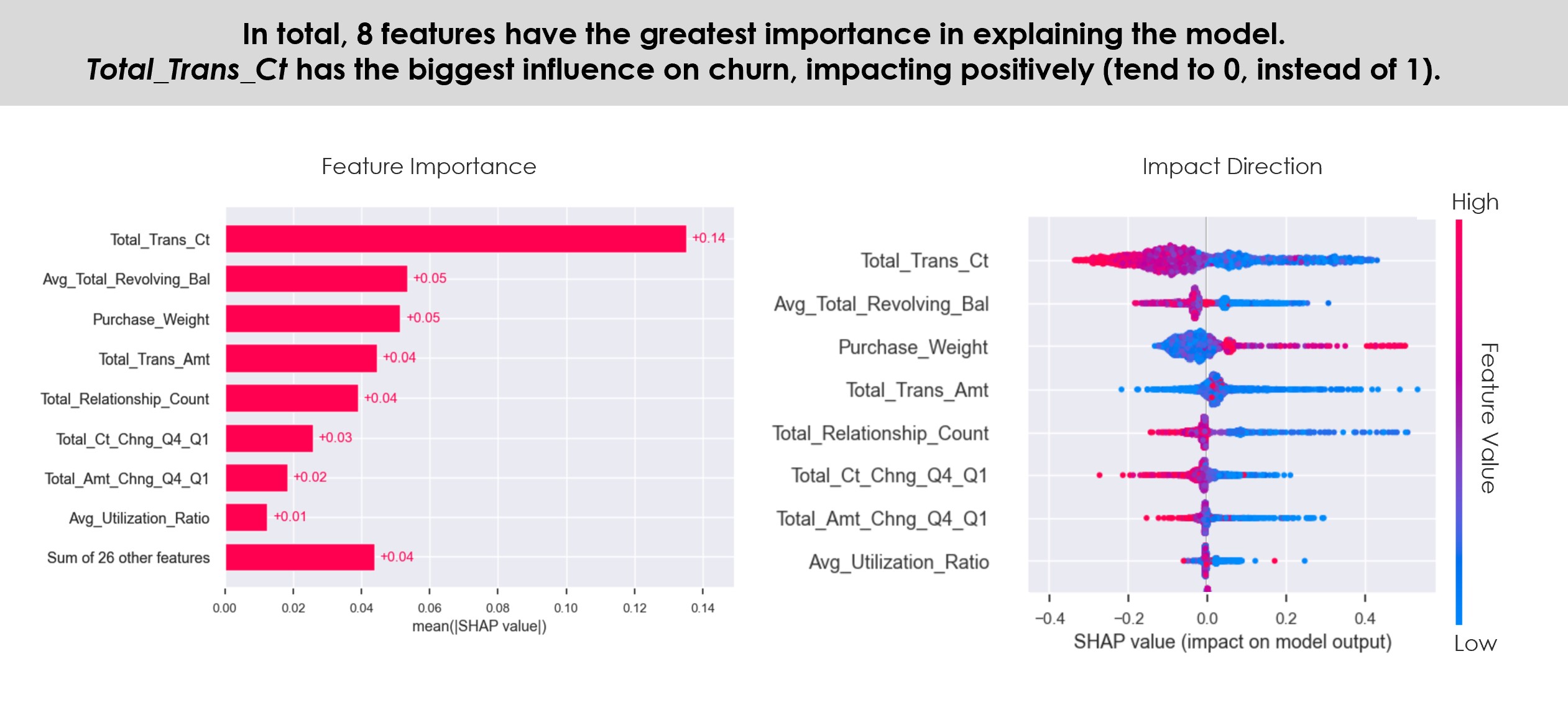
Most important, unlike many machine learning methods, especially ANN, Random Forest is not a “black box”. RF produces an index of variables ranked by their importance on the classification accuracy (Breiman, 2001), being easier to interpret the results. Because of its mixed method of Bootstrap Aggregation with Feature Randomness, is possible to measure the importance of each feature, as well as estimate the ensemble’s strength, correlation and generalization error (PE) in every tree’s split, allowing the model to be fit and validated whilst being trained (Breiman, 2001; Hastie, Tibshirani, & Friedman, 2009).
In summary, it is a very simple and complete “out of the box” algorithm. It is usually recommended before trying other methods of classification that takes more time to train and execute.
Predicting
For the regression analysis, both linear and ordinal logistic regression were performed, being the latter more suitable for predicting dependent variables in an ordinal scale presentation, such as the OCR score (McCullagh, 1980).
First, categorical variables such as late and product_category were changed into numeric variables. Product categories, in particular, were recoded into dummy variables for linear regression analysis, which did not significantly change the output, with an R-squared increasing from 0.099 (not including categories) to 0.106 (including categories). Overall, as expected, the model does not perform well in a linear regression analysis, presenting a typical mean squared prediction error of about 1.206, which is substantial when trying to predict values in a 1-5 array.
Next, the multicollinearity of the predictors has been tested in an ordinary least squares (OLS) regression analysis by checking the Variance Inflation Factor (VIF), which is the proportion of the variances in a multiple-terms model comparing to the one-term model (Gareth, et al., 2017). This collinearity analysis is required to drop any highly correlated predictors and, as expected, the extracted features total_value and delivery_precision (when using the late variable) or delivery_est_time (when not using late) were excluded for having a high VIF.
Therefore, for the ordinal logistic regression, total_value and delivery_precision was removed from the model. The other variables presented a VIF value between 1.0 and 2.0, not needing to be removed.
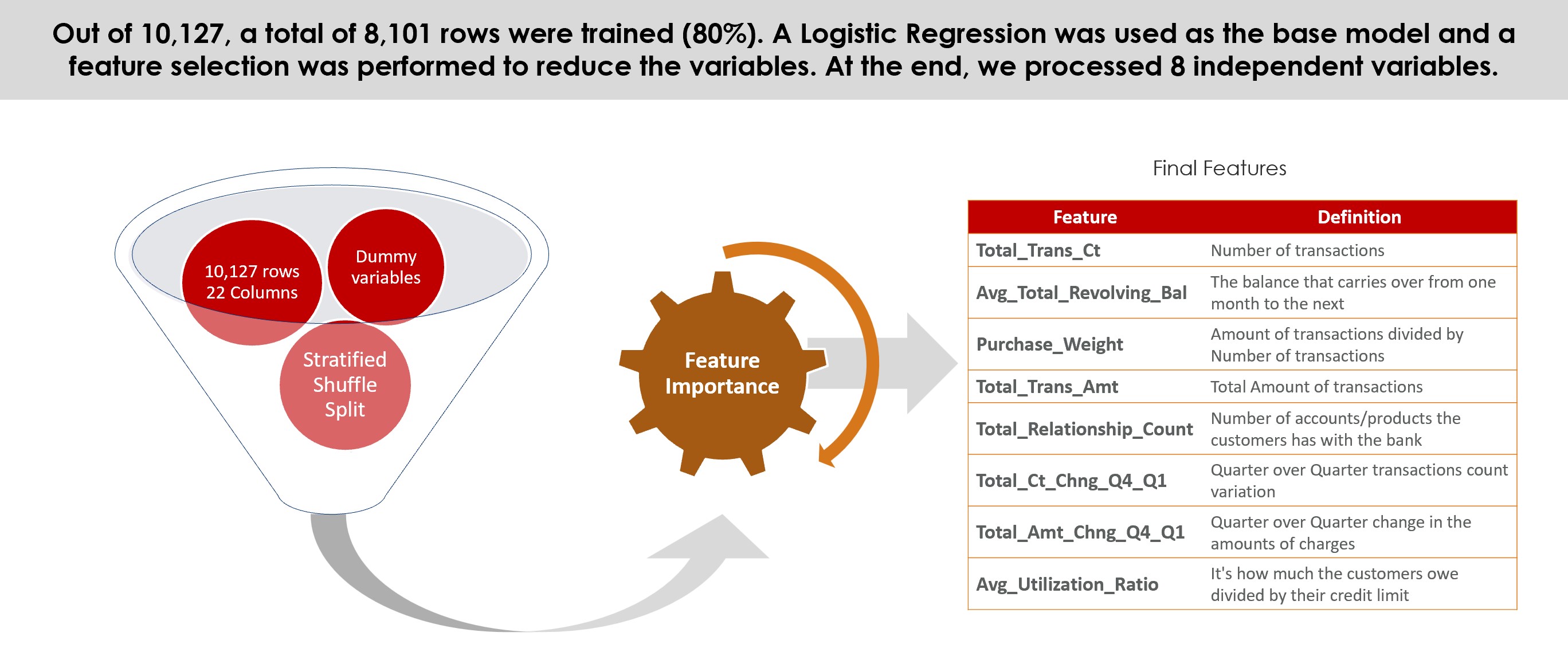
For splitting the data set into training and test sets, a model selection tool from scikit-learn library known as Stratified ShuffleSplit was used as cross-validator. It “provides train/test indices to split data into train/test sets”, returning “stratified randomised folds (…) made by preserving the percentage of samples for each class” (scikit-learn developers, 2019).
This type of split better represent the original set and potentially decreases any bias for Random Forest Regression and Classification. The proportion of training and test set size was set as 80:20. Next, the Labels and Features data sets were created, separating review_score from the other features.
A typical prediction error of about 1.20 is not at all satisfying when we are trying to predict values that range from 1 to 5.
The next step was to perform the ordinal logistic regression. The only ordinal categorical variable in the model was the dependent variable review_score, the same as in the linear regression analysis, of course. On the independent variables side, the categorical variables product_category and late were classified as factors in the SPSS Statistics procedures, while prod_value, delivery_value, descr_size, photos_qty, delivery_est_time and delivery_act_time were treated as covariates, with only descr_size and photos_qty not being continuous.
The assumption of no multicollinearity was also validated by removing total_value and delivery_precision from the model and testing the VIF of product_category dummy variables. A full likelihood ratio test was similarly performed to ensure the features would have proportional odds and other assumptions, as normally distributed error terms (residuals) and homoscedasticity are not required for ordinal logistic regression (Menard, 2010). The large sample size also helps to assume linearity of independent variables related to the log odds. Lastly, scaling through standardisation is not required for logistic regression since its own exponential function already saturates a value once it crosses the threshold.
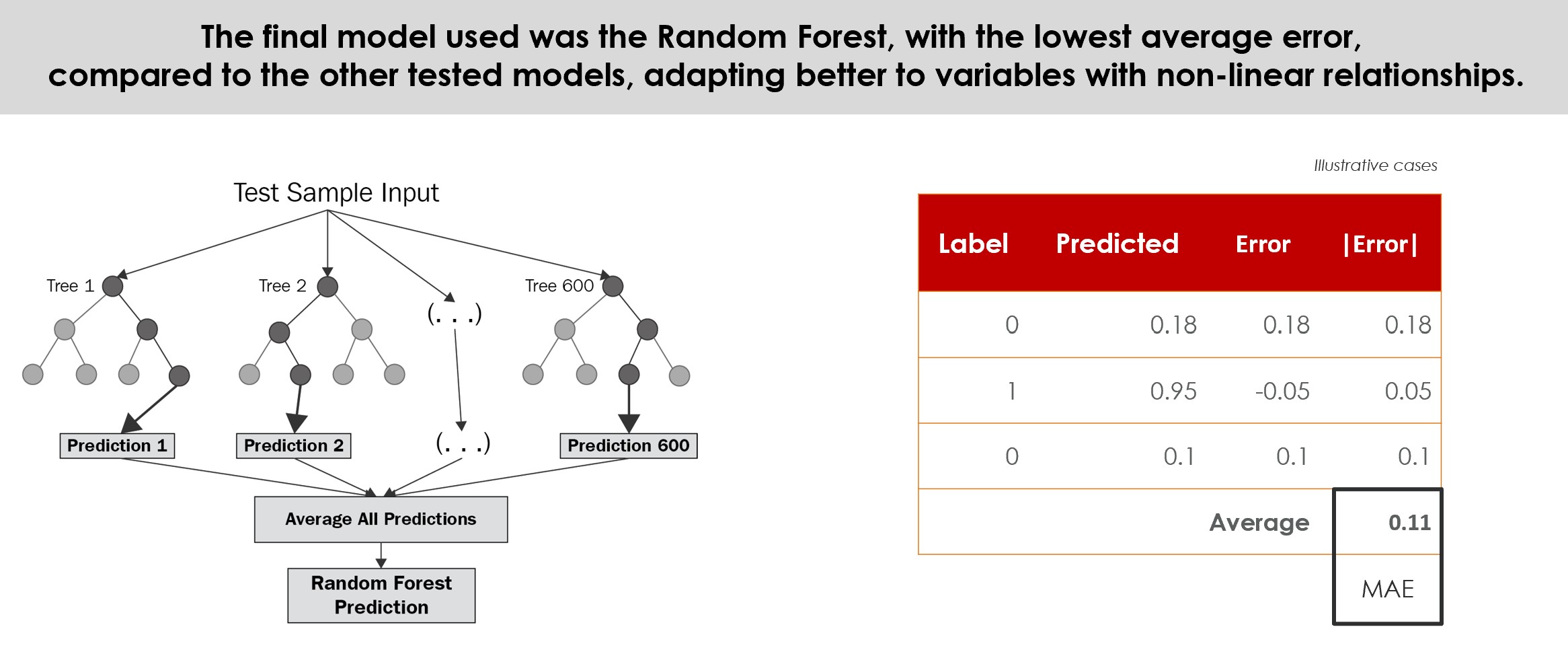
Random Forest is one of the most popular ensemble methods for supervised machine learning and is able to perform both regression and classification, “serving as an off-the-shelf procedure for data mining” (Hastie, et al., 2009). It develops a “forest” by building up a multitude of decision trees capable of handling both numerical and categorical data; and non-linear relationship parameters do not affect its performance (Breiman, 2001).
Additionally, Random Forests can handle large data sets with high dimensionalities and will correct decision tree’s potentially model overfitting through their Bootstrap Aggregation (or bagging) and Feature Randomness methods (Hastie, et al., 2009).
The advantage incurred from training the samples with the bagging method before the ensemble process is the creation of different individual learning models, trained on subparts of the same set, reducing the learning process variance before voting or adding the output at the end (Hastie, et al., 2009). In addition, Feature Randomness allows Random Forests constituent trees to use only the random subset of variables (instead of considering all variables as in a standard decision tree), reducing the correlation between trees (Breiman, 2001).
This diversification gives this research’s diverse independent variables more relevant weights according to their importance. The result of this vast amount of reasonably uncorrelated trees is a more accurate prediction performance than any of its individual component’s predictions alone (Ho, 1995), compensating the small increase of bias that comes with reducing the variance.
Typical error of 0.12 with Random Forest Classifier. Even better than Regression.
Read more
Feel free to download the repository and check how everything's working for yourself. And let me know if you have any comments.
The source code of the project is on Github and you can also see it on nbviewer.
